
VLOOKUP searches for a value in the first column of a table and returns information from another column. When it returns #N/A, it means “not found” — even if the value looks like it’s there. Here are the causes, from most to least common.
In this article
1. Extra spaces
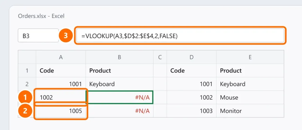
A trailing (1002 ) or leading space makes Excel treat the values as different. Clean them with the TRIM function in a helper column and paste the result as values:
=TRIM(A2)Or use it inside VLOOKUP itself: =VLOOKUP(TRIM(A2),$D$2:$E$100,2,FALSE).
2. Numbers stored as text
Codes imported from other systems often come in as text — they’re left-aligned and show a green triangle in the corner. Select the cells, click the warning and choose Convert to Number. Both columns (the lookup value and the table) must be the same type.
3. Missing FALSE at the end
The fourth argument sets the match type:
- FALSE (or 0): exact match — what you want in almost every case.
- TRUE or blank: approximate match, which requires the table sorted in ascending order and returns wrong values if it isn’t.
4. The lookup column isn’t the first one
VLOOKUP only searches the first column of the range. If the code is in column D, the range must start at D ($D$2:$E$100), and the column number counts from there (D = 1, E = 2).
5. The range “moved” when you copied the formula
Without $, the range shifts down as you drag the formula and leaves rows out. Use absolute references: $D$2:$E$100 (press F4 to add the dollar signs).
The value really isn’t there
If the value truly isn’t in the table, #N/A is correct. To show a message instead of the error:
=IFERROR(VLOOKUP(A2,$D$2:$E$100,2,FALSE),"Not found")Use XLOOKUP if you have Microsoft 365
XLOOKUP searches any column, uses exact match by default and has a built-in “if not found” argument:
=XLOOKUP(A2,D:D,E:E,"Not found")Also see what each Excel error means.
FAQ
VLOOKUP works in one row but not another.
Compare the two cells with =A2=D5 — if it returns FALSE, there’s an invisible difference (a space or type). See causes 1 and 2.
VLOOKUP between two different workbooks doesn’t work.
Keep both workbooks open while creating the formula and check that the other file’s path is right. If the source file was moved, update it under Data › Edit Links.
The formula shows instead of the result.
The cell is formatted as text or Show Formulas is on — see Excel formula not calculating.